Lead Scoring Analysis and Segmentation

Note: Documentation available on the GitHub Repository is currently in Spanish. It will be soon updated to English.

• Launch Lead Scoring Analyzer Web App!

1. Introduction

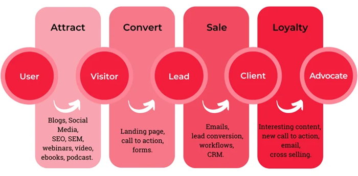
The client for this project is an online teaching company that offers a high-value online course designed to train professionals in the data science sector. The company advertises this course on various websites and search engines. When people visit the website—promoted effectively by the marketing department—they may browse the course, fill out a form, or watch related videos. If they provide their email address or phone number through a form, they are classified as a lead. Additionally, the company also acquires leads through referrals from past clients.

Once these leads are acquired, the sales team begins reaching out via calls, emails, and other forms of communication. However, while some leads convert into customers, most do not, leading to inefficiencies that negatively impact the company’s profitability.

Notes:

• This article presents a technical explanation of the development process followed in the project.
• Source code can be found here.
• You can also test the Lead Scoring Analyzer web application.

2. Objectives

The main objective is to analyse the historical leads information of the company to propose potential actions that will increase the overall turnover and reverse the low conversion rate at which the company is operating. To achieve this goal, we will create advanced analytical assets such as:

• Lead segmentation model: This tool will help to identify the key customer groups interested in the product, enabling the sales team to tailor marketing efforts effectively for each identified segment.
• Predictive lead scoring model: It will assist the sales team in identifying potential customers who are most likely to convert into final clients, as well as leads that are not economically viable to pursue.

3. Understanding the problem

Nowadays, there are basically two main methodologies that a company can apply in order to get a final client. These are outbound and inbound marketing models. Outbound marketing is known for using traditional methods to reach potential buyers, such as advertisements, events, product samples, and phone calls. In contrast, inbound marketing focuses on attracting consumers to the company, encouraging them to seek out more information about a product or service on their own.

Outbound strategies are often seen as more aggressive, requiring consistent and repeated efforts from sellers. In inbound marketing, however, sellers typically engage only after the customer has made the first move.

Inbound marketing guarantees that when executed properly, the company will reach a more targeted audience with higher buying potential. As a result, investing in inbound marketing is more economical, often yielding a higher return on investment.

One of the challenges associated with inbound marketing is that the number of generated leads exceeds the capacity of the sales channels, leading to several issues:

• Conflicts between marketing and sales departments: The marketing department expects a higher conversion rate from the large pool of leads, while the sales department is frustrated by the low quality of these leads, feeling they are wasting valuable time.
• Saturation of the sales channels: The sales team can only handle a limited number of leads effectively.
• Low conversion rate: As a result, the company’s performance is significantly below potential, which could be improved with proper lead management based on Machine Learning optimization.

For all the reasons mentioned above, it is essential to implement some form of lead prioritization to achieve higher conversion rates. The assets we are developing for the company—specifically the predictive lead scoring and customer segmentation algorithms—are designed to address this need. These tools will enable the company to identify the highest-quality leads and recognize key customer segments, thereby refining their approach strategy for each group.

4. Project Design

4.1 Methodology

The project has been designed with a multi-step methodology, which is summarized in the figure bellow.

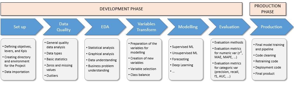
The process for this project consists of two main stages: the development phase and the production phase.

The development phase begins with the set up and data importation, followed by a thorough data quality review. Next, an exploratory data analysis is conducted to uncover key insights. The variable transformation step involves selecting the most relevant variables that impact the problem and applying the necessary transformations. Following this, models are implemented for both the predictive and segmentation algorithms. During the evaluation process, all metrics are thoroughly tested.

In the production phase, the models are prepared for deployment, ensuring that the code is optimized for production. Additionally, a retraining script is created during this stage to facilitate future updates.

4.2 Levers

The main levers for this project are summarized below:

• Leads: Understanding general information about the leads the company receives is crucial for optimizing future marketing campaigns.
• Conversion rate: This metric indicates the ratio at which leads convert into customers. Our goal is to maximize this metric to boost the company’s profits.
• Commercial channels optimization: The sales department has various channels for communicating with leads, including phone calls, SMS, emails, web chat, and a subcontracted lead management company. Optimizing these channels is key to improving overall efficiency.

4.3 KPIs

The KPIs that results from the above-mentioned levers are the following:

• Lead-to-customer conversion rate (CR): Ratio at which leads convert into customers. It is defined as: $$ \textup{CR}[\%] = \frac{\textup{N}_\textup{C}}{\textup{N}_\textup{L}}\cdot 100, $$ where $\textup{N}_\textup{C}$ and $\textup{N}_\textup{L}$ are de number of final customers and leads, respectively.
• Sales department workload $(\textup{N}_\textup{L})$: Number of potential customers to be managed by the sales team.
• Loss investment in unconverted lead management $(\textup{Cost}_{\textup{not conv leads}})$: Cost of commercial efforts directed toward potential customers who ultimately do not purchase the company’s product. It is defined as: $$ \textup{Cost}_{\textup{not conv leads}} = \left( \textup{N}_\textup{L} - \textup{N}_\textup{C} \right) \cdot \textup{Cost}_{\textup{leads}}, $$ where $\textup{Cost}_{\textup{leads}}$ is the cost per lead arising from commercial and marketing actions.
• Sales profit (SP): Net profit obtained from the sales of the online course. It is defined as: $$ \textup{SP}[$] = \left( \textup{Price}_{\textup{prod}} - \textup{Cost}_{\textup{leads}} \right) \cdot \textup{N}_\textup{C} - \textup{Cost}_{\textup{not conv leads}}, $$ being $\textup{Price}_{\textup{prod}}$ the price of the online course.

4.4 Entities and Data

The most relevant entities from which we can obtain data are summarized below:

• Leads: Leads historical data is provided by the client in a .csv file, which contains information about 37 different features for 9240 different leads.
• Product: The product that the company is trying to sell is a high-value online course design to train proffesionals in the data science sector. Its price is 49.99$.
• Commercial channels: The main commercial channels are phone calls, sms, emails, web chat, ad campaings, and a subcontracted lead management company. The lead management average cost is estimated at 5$ per lead.

Before conducting any analysis or data transformation, it is crucial to set aside a portion of the dataset for validation purposes. This reserved data is used to validate the models after they have been trained and tested on the remaining data. Specifically, 30% of the dataset is saved for validation, while the remaining 70% is used for training the models.

5. Data Quality

In this stage of the project, general data quality correction processes have been applied, such as:

• Data renaming.
• Type correction.
• Proper selection of the most relevant data for the project.
• Analysis of nulls and duplicated registers.
• Analysis of numerical and categorical variables.
• Discretization of variables.
• Creation of new variables.

The entire process can be consulted in detail here.

6. Exploratory Data Analysis

The aim of this phase of the project is to identify trends and patterns that can be transformed into insights, providing valuable information for our project. To achieve this, we perform various statistical evaluations and create graphical representations.

In order to guide this process, a series of seed questions are proposed to serve as a basis for the analysis.

6.1 Seed questions

Regarding Leads:

• Q1: What are the main demographic profiles in the company’s lead database?

Regarding Conversion Rate:

• Q2: What is the current lead-to-customer conversion rate?
• Q3: What factors have the most significant impact on lead-to-customer conversion?

Regarding Commercial and Marketing Channels:

• Q4: How are the company’s commercial and marketing channels performing?
• Q5: From which sources is the company attracting potential customers? Which sources are the most promising?
• Q6: Which demographic profile should be the primary focus of marketing efforts?
• Q7: What percentage of leads are open to receiving communications via email or phone calls?
• Q8: How effective have the company’s advertising campaigns been?
• Q9: How well is the current lead magnet performing?

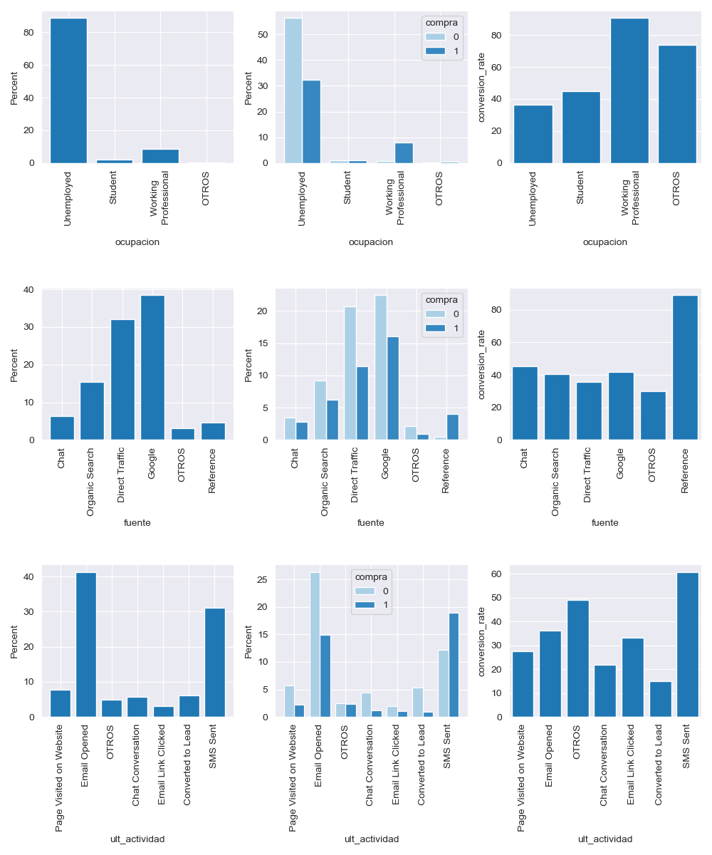
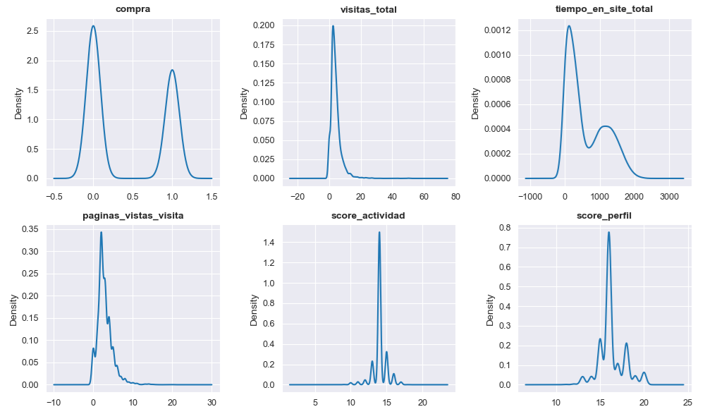
6.2 Some results obtained through the EDA

These are some of the results that we have obtained by performing the exploratory Data Analysis (EDA) for both categorical and numerical variables that are present in the dataset.

A more detailed analysis of this stage can be found here.

6.3 Insights obtained through the EDA

Once the exploratory data analysis has been conducted, the following insights have been obtained:

Leads:

• Insight 1: The mayority of the potential customers that are interested in the company are unemployed, particularly 88.84% of the leads.
• Insight 2: Only 8.64% of the leads are working professionals.
• Insight 3: The number of leads coming that comes from students is very low. It only represents 2.05% of the leads.

Lead-to-customer conversion rate:

• Insight 4: The current conversion rate of the company is 41.70%.
• Insight 5: Working professionals presents the highest conversion rate of 90.74%.
• Insight 6: Unemployed leads, which are the largest group, have a low conversion rate of 36.52%.
• Insight 7: Almost all leads that comes from the source Reference are converted into customers (89.19% conversion rate). However, only 4.56% of leads come from this source.

Commercial and marketing channels:

• Insight 8: It is observed that 99.98% and 91.07% of the leads do not want to receive phone calls nor emails, respectively. Therefore, the mayority of people that visit the website are not interested in the product.
• Insight 9: Email marketing campaigns have untapped potential, since last activity of 41.33% of total number of leads was opening an email but only 36.15% of them were finally converted. Only 14.9% of leads who want to be contacted by email end up converting into paying customers.
• Insight 10: SMS campaigns have proven to be highly effective, boasting a conversion rate of 60.82%.
• Insight 11: Most potential customers were not interested in receiving a free copy of the lead magnet. Those who did show interest are primarily unemployed and downloaded it mainly from the landing page.
• Insight 12: Converted leads spend a median of 16 minutes on the website and visit an average of 2.5 pages per session. In contrast, non-converted leads spend a median of only 6 minutes on the site.

6.4 Recommended actions

Actions to improve leads’ management:

1. Enhance the quality of survey or form questions to gather more user inputs and reduce the occurrence of NaN or default (‘Select’) values.
2. Collect timestamps for website visits to enable seasonality analysis and implement cookies to track and identify users as they navigate different pages on the website.
3. Develop a new lead segmentation algorithm that categorizes the company’s diverse lead profiles, enabling the identification of the best-fitting group for each new lead. This will allow for more personalized commercial actions.

Actions to improve lead-to-customer conversion rate:

1. Implement a predictive lead scoring algorithm that identifies individuals most likely to convert into paying customers. This will reduce the sales team’s workload allowing them to focus more time on engaging with the most promising leads.

Actions to improve commercial and marketing channels performance:

1. Enhance the content strategy across the website, lead magnet, and emails to attract more traffic and increase user engagement. Focus on creating tailored content specifically for working professionals interested in the data science sector.
2. Develop a referral program to motivate existing customers to recommend the course to their friends, family, and colleagues.
3. Allocate more resources to acquiring leads through ‘Reference’ channel, as they demonstrate the highest conversion rate.
4. Boost investments in SMS campaigns, given their strong performance.

7. Variable transformation

At this stage of the project, various variable transformation techniques are applied to ensure they meet the requirements of the algorithms used in the modeling phase.

As outlined during the exploratory data analysis, two distinct models will be developed:

1. A lead segmentation model to assist sales and marketing teams in identifying different lead profiles within the company.
2. A predictive lead scoring model to pinpoint individuals most likely to convert into paying customers.

In both models, categorical variables must be transformed into numerical ones. Since the categorical cariables in the dataset are all nominal, the one-hot encoding technique is employed for this purpose.

For the lead segmentation model, an unsupervised machine learning algorithm is recommended, specifically the KMeans algorithm. This clustering-based algorithm is highly sensitive to the scales of different features because it relies on distance calculations. Therefore, rescaling techniques must be applied to ensure that all features are on the same scale. Given the decision to apply one-hot encoding to categorical variables, the most appropriate rescaling technique in this case is min-max scaling, which will transform feature values to a scale between 0 and 1.

For the predictive lead scoring model, a supervised machine learning algorithm is recommended. Among the various classification algorithms available, the most promising candidates are logistic regression, random forest, XGBoost, and LightGBM. We will analyze these options in more detail later.

Additionally, we need to decide whether to apply feature discretization or binarization. Considering that the project’s primary focus is on prediction accuracy rather than interpretability, and given that one of the models is based on a segmentation algorithm, neither discretization nor binarization will be applied.

Lastly, it is important to note that class balancing processes are not necessary for this project, as the dataset contains a sufficiently significant representation of both classes (converted=1, converted=0).

More details can be found here.

8. Lead segmentation model

At this stage, after completing data quality checks, exploratory data analysis, and variable transformation, we are ready to develop the lead segmentation model. As mentioned earlier, an unsupervised machine learning model will be used for this purpose, specifically the KMeans algorithm, which has demonstrated strong performance in the clustering process. By implementing this model, we aim to uncover new insights that can enhance the company’s sales and marketing strategies.

More details about the lead segmentation model can be found here.

8.1 Selecting the number of segments

In order to identify the optimal number of clusters in the KMeans algorithm, we apply 4 different methods. The result are shown in the figure below.

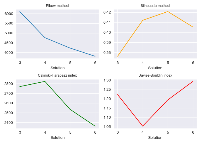
• Elbow Method: This method typically identifies the optimal number of clusters by selecting the point where the curve bends or “elbows,” indicating diminishing returns in reducing within-cluster variance. However, in this case, the chart shows only a linear decrease, offering little useful guidance for cluster selection.

• Silhouette Method: This metric measures how similar each point is to its own cluster compared to other clusters. Values closer to 1 indicate better-defined clusters. Here, a segmentation of 4 to 5 clusters appears optimal based on this method.

• Calinski-Harabasz Index: This index evaluates cluster separation, with higher values indicating better-defined clusters. According to this method, a segmentation into 3 or 4 clusters is likely the best.

• Davies-Bouldin Index: This index assesses the average similarity ratio of each cluster to its most similar cluster, with lower values indicating better clustering. For this analysis, a segmentation of 4 clusters is preferred based on this index.

It is important to note that an iterative process was applied before arriving at the final charts. The procedure involved the following steps:

1. Initially, charts for the four methods mentioned above were generated. Based on this data, a fixed number of clusters was selected.
2. The KMeans algorithm was then applied with this fixed segmentation, and the values for each variable were analyzed.
3. Typically, initial segmentations revealed some inconsistencies, leading to the elimination of certain variables and testing different cluster configurations.
4. Steps 1 through 3 were repeated several times until a final, consistent cluster segmentation was achieved.

After completing this process, it was determined that a 4-cluster segmentation provided the most meaningful business insights.

8.2 Segment profiling

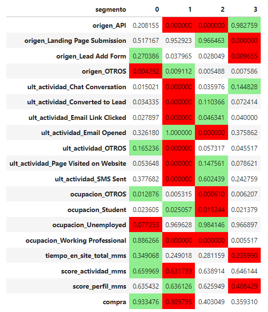
Once the optimal number of clusters and the most relevant segmentation variables have been selected, the model is trained and executed, assigning each lead to one of the four existing clusters.

To understand the business implications, average values for each variable used in the model has been calculated, allowing us to identify the most distinguishing characteristics of each segment. This is shown in the table below.

8.3 Segment analysis

After analysing the above results, the most differential characteristics for each segment are identified and presented.

Segment 0: Super high-quality Leads

• Origin: Lead Add Form.
• Last activity: Non categorize.
• Occupancy: Working Professionals.
• Largest time spent on the website.
• Great conversion rate. Nine out of ten leads in this segment end up buying the company’s product.

Segment 1: Very low-quality Leads

• Origin: Landing Page Submission.
• Last activity: Email opened.
• Occupancy: Students and unemployed.
• Very low time spent on the website.
• Worst conversion rate group.

Segment 2: Medium-quality Leads

• Origin: Landing Page Submission.
• Last activity: SMS sent.
• Occupancy: Unemployed.
• They spend some time on the website.
• Moderate conversion rate.

Segment 3: Low-quality Leads

• Origin: API.
• Last activity: Chat conversation.
• Occupancy: Unemployed.
• Very low time spent on the website.
• Low conversion rate.

8.4 Segmentation insights

1. The company’s most valuable leads are working professionals who arrive through the lead form submission.

2. While SMS campaigns are generally effective, they should be targeted more precisely:

• Focus on working professionals from API sources who spend above-average time on the website.
• Avoid sending SMS to leads from Landing Page Submissions who spend minimal time on the site, as they represent the lowest quality leads and divert resources from more promising campaigns.

3. The live chat feature primarily attracts low-quality leads. The company should consider reallocating resources from this service and, for leads from API sources, prioritize email marketing and SMS campaigns instead.

9. Predictive lead scoring model

A predictive lead scoring model is developed using a supervised machine learning approach. At this stage of the project, several algorithms are tested, including logistic regression, random forest, XGBoost, and LightGBM. Each algorithm is analyzed with an extensive range of hyperparameters to ensure optimal predictive performance. The implementation of this model will enhance customer identification, thereby increasing the conversion rate (CR) and reducing marketing costs.

More details for the predictive lead scoring model can be consulted here.

9.1 Variable selection for predictive model

Several variable selection methods were tested to identify the most useful features for the predictive model. The primary methods considered were mutual selection, recursive feature elimination, and permutation importance. Among these, permutation importance proved to be the most accurate for this case and aligned well with the variable selection used in the lead segmentation model. The results are displayed in the image below.

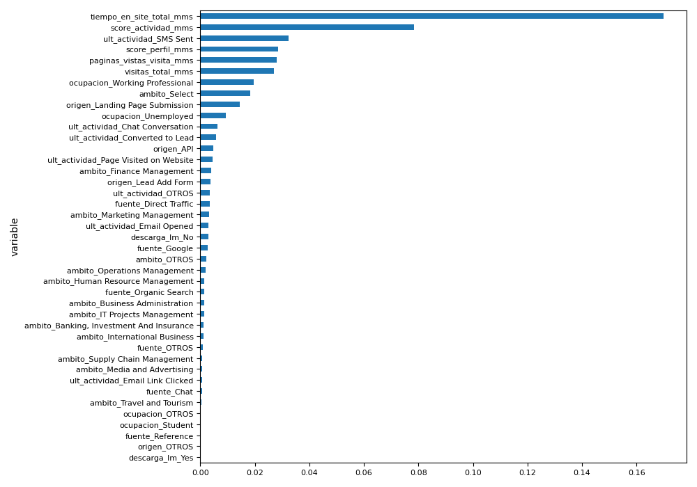
Based on the permutation importance method, the 20 most relevant variables were selected for the predictive model. Additionally, the correlations between these variables were examined, and highly correlated ones were removed. While strong correlations do not typically hinder tree-based algorithms, they can negatively impact the performance of other algorithms, such as logistic regression.

More details here.

9.2 Model selection

Different combinations of hyperparameters are tested for each of the algorithms and the ones with the best AUC (Area under Curve) scoring are collected. On the other hand, all of the combinations are tested with the cross-validation method in order to ensure a good stability in the models. The performance of these algorithms is tested with three methods, which are cumulative gains curve, lift curve, and ROC curve.

Roughly speaking, the cumulative gain curve measures the effectiveness of a classification model by showing the proportion of true positives, while the lift curve shows the ratio of the model’s performance to random performance, which helps to understand how much better the model is compared to random guessing. The ROC curve is used to evaluate the trade-off between the true positive rate (sensitivity) and the false positive rate at various threshold settings.

The cumulative gains and lift curves focus on how well the model identifies positives within a sorted population, while the ROC curve evaluates the overall discrimination capability of the model across all thresholds. The results are shown in the figure below.

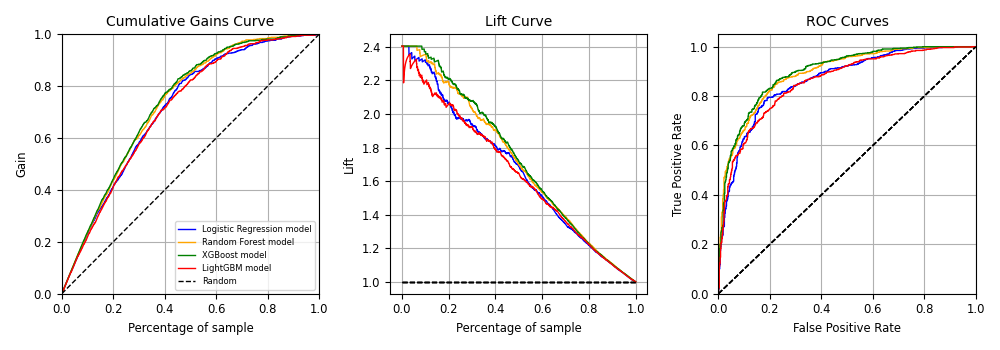
The XGBoost algorithm presents the best performance in the three charts, however, the results are pretty similar for all of them. Therefore, it is decided to implement the logistic regression algorithm for the project due to the following reasons:

1. Its predictive ability closely matches that of the random forest, XGBoost, and LightGBM models.
2. It offers greater interpretability compared to the more complex tre-based algorithms.
3. Being a simpler model, it is easier to maintain and quicker to train, retrain, and execute.
4. Its mathematical simplicity allows for easy migration to the platforms and software used by the company.

Thus, the logistic regression algorithm is used with the following hyperparametrization:

• C = 1
• n_jobs = -1
• penalty = ’l1'
• solver = ‘saga’

9.3 Optimal discrimination threshold for maximizing ROI

Once the predictive model is trained and tested, the next step is to specify the optimal threshold that determines whether a lead is classified as a potential customer (1) or not (0) based on the model’s score. To achieve this, a method focused on maximizing ROI is implemented. This method determines the optimal threshold using confusion and impact matrices, which are defined as follows.

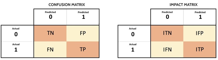
• Confusion matrix: This matrix is used to describe the performance of a classification model. It shows the actual versus predicted classifications and helps to identify how often the model is correctly and incorrectly predicting each class. The output “TN” stands for True Negative which shows the number of negative examples classified accurately. Similarly, “TP” stands for True Positive which indicates the number of positive examples classified accurately. The term “FP” shows False Positive value, i.e., the number of actual negative examples classified as positive; and “FN” means a False Negative value which is the number of actual positive examples classified as negative.
• Impact matrix: This matrix is used to quantify the impact or cost associated with the different types of errors made by a model, such as false positives and false negatives. Unlike the confusion matrix, which counts occurrences, the impact matrix assigns a numerical value to the consequences of these outcomes. The output “ITN” stands for Impact of True Negative which shows the economic impact of not to carry out any commercial actions on those leads that were not going to buy the product. Similarly, “ITP” stands for Impact of True Positive which indicates the net profit obtained from commercial actions on customers who end up buying the course. The term “IFP” shows Impact of False Positive value, i.e., the opportunity cost of not having carried out commercial actions on leads who would have become customers. Finally, “IFN” means a Impact of False Negative value which represent the economic cost of commercial actions carried out on a lead that finally does not buy the company’s product.

Therefore, by calculating the confusion matrix and multiplying it by the economic impact matrix for each possible value of the discrimination threshold, it becomes possible to determine which threshold maximizes the resulting function and, consequently, the company’s ROI. The results are shown in the image below.

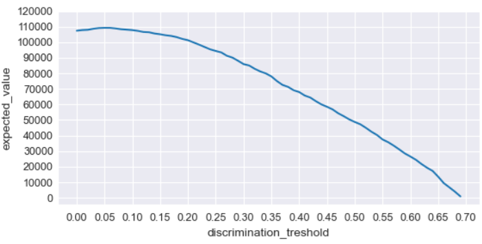
In this case, the discrimination threshold value that provides the higher return on investment for the company is 0.05.

10. Evaluation of the predictive lead scoring model

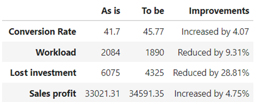
Finally, the model has been tested on a batch of 2084 leads never seen before by the model (the validation dataset that we reserved at the beginning). By applying the developed lead scoring predictive model, the company has been able to:

1. Increase its conversion rate from 41.70% to 45.77%.
2. Reduce by 9.31% the workload to be managed by the sales department.
3. Reduce by 28.81% the loss in investments.
4. Increase its sales profit by 4.75%.

The evaluation results can be found here.

11. Retraining and Production scripts

After successfully developing, training, and evaluating both segmentation and predictive models, the final stage of the project involves organizing and optimizing the entire process. This is accomplished by compiling all necessary processes, functions, and code into two streamlined Python scripts:

• Retraining Script: This script is designed to automatically retrain all developed models with new data as needed, ensuring that the models remain accurate and up-to-date.

• Production Script: This script executes all models and generates the desired results, ensuring a smooth transition from development to production.

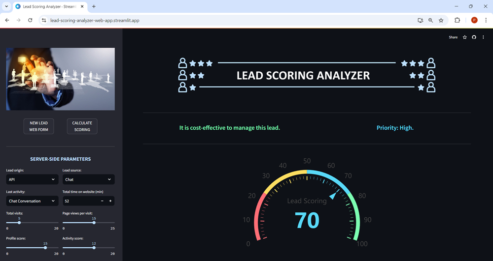
12. Model deployment. Web app creation

To maximize the value of the developed machine learning models, it is essential to seamlessly deploy them into production so that employees can start utilizing them to make informed, practical decisions.

To achieve this, a prototype web application has been designed. This web app gathers internal data from the company for each lead, as well as information provided by the customer through a web form application.

• Launch Lead Scoring Analyzer Web App!

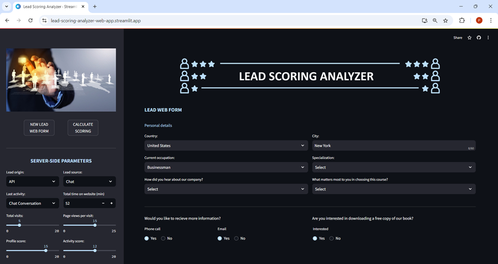
Once the data is entered, users can click the CALCULATE SCORING button, which triggers the predictive lead scoring model to process the data. The application will then return the final scoring for the lead, along with some indications about this potential customer.

The necessary files for the creation of the web app can be found here.