Sales Forecasting for a Retail Company

Note: Documentation available on the GitHub Repository is currently in Spanish. It will be soon updated to English.

1. Introduction

The client for this project is a large retailer based in the United States. The company has identified issues in its warehouse operations, leading to losses and stock-outs for several products. The objective is to implement a forecasting model using artificial intelligence algorithms to predict the appropriate stock levels for at least the next 8 days. This initiative aims to enhance operational efficiency and increase the company’s profitability.

Notes:

• This article presents a technical explanation of the development process followed in the project.
• Source code can be found here.

2. Objectives

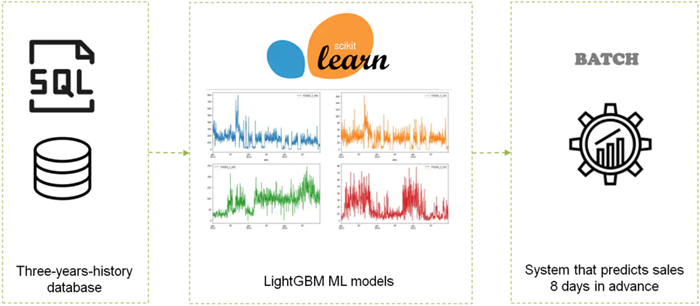
The primary objective is to develop a forecasting model utilizing a set of machine learning algorithms to predict sales for the next 8 days at the store-product level. These algorithms are trained using the extensive three-year history available in the retail company’s SQL database, employing massive modeling techniques to ensure accuracy and reliability.

3. Understanding the problem

Forecasting is one of the most widely used techniques in the data science field due to its significant impact on a company’s balance sheet and its potential to greatly enhance overall performance. Some of the mayor beneficts are summarized below:

• Inventory optimization: Forecasting helps predict demand more accurately, reducing overstock and stock-outs. This leads to better inventory management, minimizing costs and improving cash flow.

• Improved customer satisfaction: By anticipating demand, the company can ensure products are available when customers want them, enhancing the shopping experience and increasing customer loyalty.

• Better decision-making: Forecasting provides data-driven insights, enabling more informed decisions about pricing, promotions, and product launches, ultimately improving profitability.

• Resource allocation: Forecasting helps in planning staffing, logistics, and marketing efforts, ensuring resources are allocated effectively to meet anticipated demand.

• Competitive advantage: Companies with better forecasting capabilities can respond more quickly to market changes, offering them an edge over competitors.

In this context, traditional sales forecasting methods have been reliable for decades. However, with the advent of machine learning algorithms, it is now possible to implement powerful forecasting models using a data science approach. These modern techniques enable the prediction of product or service demand over a specified future period by leveraging historical company data. Compared to traditional forecasting methods, a machine learning approach offers several advantages:

• Accelerated data processing speed
• Automated forecast updates based on recent data
• Enhanced data analysis capabilities
• Identification of hidden patterns in data
• Greater adaptability to changes

For this project, an innovative forecasting model has been developed, utilizing massive and scalable machine learning techniques.

4. Project Design

4.1 Methodology

The project has been designed with a multi-step methodology, which is summarized in the figure bellow.

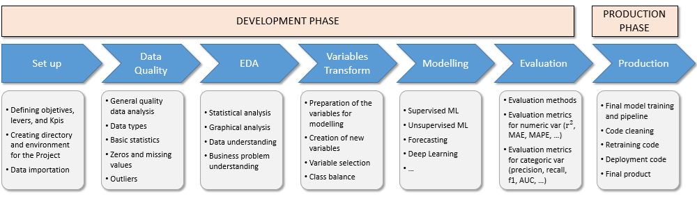
The process for this project consists of two main stages: the development phase and the production phase.

The development phase begins with the set up and data importation, followed by a thorough data quality review. Next, an exploratory data analysis is conducted to uncover key insights. The variable transformation step involves selecting the most relevant variables that impact the problem and applying the necessary transformations. Following this, the forecasting model is implemented based on machine learning algorithms. During the evaluation process, all metrics are thoroughly tested.

In the production phase, the model is prepared for deployment, ensuring that the code is optimized for production. Additionally, a retraining script is created during this stage to facilitate future updates.

4.2 Project scope, entities, and data

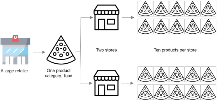
This project is developed using data from a three-year SQL database of a large American retailer. However, due to the computational constraints of the available equipment, the project’s scope is limited to forecasting sales for ten products that belong to a sigle category (food) in two different stores. Nevertheless, the system is fully scalable and can be extended to predict sales for additional products, categories, and stores by simply adjusting the relevant parameters.

The most relevant entities from which we can obtain data are summarized below:

• Store id: It shows the identification number associated with the store at which the product are sold.
• Item id: Identification number for each of the items that the company offers.
• Operation day: Code for the day when a certain product is sold.
• Number of sales: The quantity of items sold each day for each store, as recorded in the dataset.
• Sell price: Price at which the items are sold.

Before conducting any analysis or data transformation, it is crucial to set aside a portion of the dataset for validation purposes. This reserved data will be used to validate the models after they have been trained and tested on the remaining data. Since this is a forecasting project, the reserved data must be in chronological order (time series) to accurately test the model’s performance. Therefore, the data from the last month, December 2015, has been extracted and will be used as a validation later.

4.3 Forecasting-related problems approach

Hierarchical Forecasting:

In forecasting models, it is common to encounter time series data that follows a hierarchical aggregation structure. In the retail market, for instance, sales data for a Stock Keeping Unit (SKU) at a store often rolls up into various category and subcategory hierarchies. In such cases, it’s essential to ensure that the sales forecasts are consistent when aggregated to higher levels. To achieve this, a hierarchical forecasting approach is employed, which generates coherent forecasts (or reconciles incoherent ones). This approach allows individual time series to be forecasted independently while maintaining the relationships within the hierarchy.

The major problems when generating a forecasting model are the following:

• There are different levels of hierarchies in the commercial catalog.
• It may be interesting to predict sales at different levels.
• Since the forecasts are probabilistic, predictions at different levels will not match exactly.

A hierarchy forecasting approach offers different methods to solve these problems. The most common ones include:

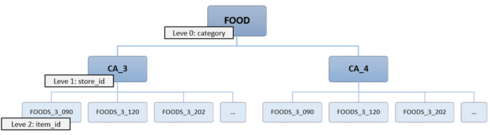
• Bottom-up: This method begins by forecasting at the most granular level of the hierarchy (e.g., items in level 2) and then aggregates these forecasts up to higher levels (e.g., stores in level 1 and finally food in level 0). It provides detailed and localized insights, capturing specific trends and patterns. However, the aggregation process may introduce inconsistencies or misalignment at higher levels if the individual forecasts are not well-calibrated.

• Top-down: This method begins with forecasting at the highest level of the hierarchy (e.g., food in level 0) and then distributes the forecast down to lower levels (e.g., stores in level 1 and finally items in level 0). The roll down is done by mantaining the percentage representation of each subcategory from the raw data. This system ensures that the overall forecast is consistent with the broader organizational targets and constraints. However, it might overlook specific local variations or nuances that are important at lower levels.

• Hybrid: This method combines elements of both bottom-up and top-down approaches. For example, it might start with a top-down forecast to set high-level targets and then refine the forecast using bottom-up methods to adjust for local details. It aims to balance the accuracy of detailed forecasts with the consistency of high-level targets, potentially improving both overall alignment and granularity. However, implementing a hybrid approach can be complex, as it requires coordination between different forecasting processes and levels of the hierarchy.

In this project, a bottom-up approach is implemented for hierarchical forecasting, where the models are developed at the most granular level, specifically the store-product level.

Intermittent demand:

Intermittent demand, or sporadic demand, occurs when a product experiences multiple periods of zero sales. This issue can arise from two primary causes:

• The product was in stock but no sales occurred.
• The product was out of stock, preventing any sales.

The source of these zero values can sometimes be unclear, leading to noise and making it difficult for the model to generate accurate predictions.

To address intermittent demand, several solutions can be employed:

• Getting the inventory information: It helps us to generate stock-out features that allow the algorithms to discriminate the cause of the zero values.

• Model at a higher hierarchical level: If the inventary information and/or stock-out marks are not available, another possible approach is to model at a higher hierarchical level, especially if the products are in very low demand.

• Create synthetic features: It is also possible to create synthetic features that try to identify whether or not stock-outs have occurred.

• Machine learning forecasting: Employing forecasting methods based on machine learning techniques, which are less sensitive to these problems than classical approaches.

• Advanced methodologies: Lastly, there is some more advanced methodologies such as croston method and specialized machine learning models can predict the probability of zero sales on certain days.

In this project, since inventory and stock-out information are not available, synthetic features will be created based on business rules to indicate potential stock-out scenarios.

Huge amount of Stock Keeping Units (SKUs):

In practical applications, particularly in sectors like retail and e-commerce, there are often thousands of different products that need to be modeled to predict sales levels accurately. Given the vast number of SKUs, the desired level of temporal aggregation (e.g., hourly, daily, weekly), the volume of historical data, and the available computational resources, the modeling process can become computationally infeasible. This complexity can challenge even advanced systems and may necessitate the use of scalable approaches or optimization techniques to manage the modeling workload effectively.

In this context, several solutions can be employed:

• Adopt Machine Learning Forecasting: Machine learning models, once trained, can generate forecasts much faster than traditional methods, improving efficiency.
• Utilize Fast Algorithms: Implement faster algorithms like LightGBM, which are optimized for speed and scalability.
• Hierarchical Modeling: Model at a higher hierarchical level and apply top-down reconciliation techniques to estimate forecasts for lower levels, balancing detail and computational demands.
• Leverage Big Data Technologies: Employ big data techniques, such as using powerful cloud computing resources or big data clusters, to handle large datasets and complex models efficiently.

Consequently, for the reasosns explained above, a forecasting model based on a machine learning approach and a LightGBM tree-based algorithm architecture has been developed in this project.

5. Data Quality

In this stage of the project, general data quality correction processes have been applied, such as:

• Data renaming.
• Type correction.
• Proper selection of the most relevant data for the project.
• Analysis of nulls and duplicated registers.
• Analysis of numerical and categorical variables.
• Discretization of variables.
• Creation of new variables.

The entire process can be consulted in detail here.

6. Exploratory Data Analysis

The aim of this phase of the project is to identify trends and patterns that can be transformed into insights, providing valuable information for our project. To achieve this, we perform various statistical evaluations and create graphical representations.

In order to guide this process, a series of seed questions are proposed to serve as a basis for the analysis.

6.1 Seed questions

Regarding sales:

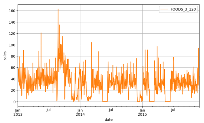
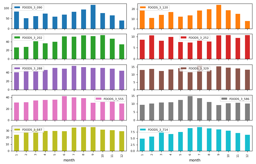
• Q1: How has the company’s sales performance evolved over time?
• Q2: How about the sales per product?
• Q3: How are product sales performing across different stores?
• Q4: Are product sales consistent over time, or are there periods with zero demand? If so, is this due to stock-outs, or are the products simply not selling during those periods?
• Q5: What is the seasonality pattern in sales? How do sales vary by month and by day of the week?

Regarding sell price:

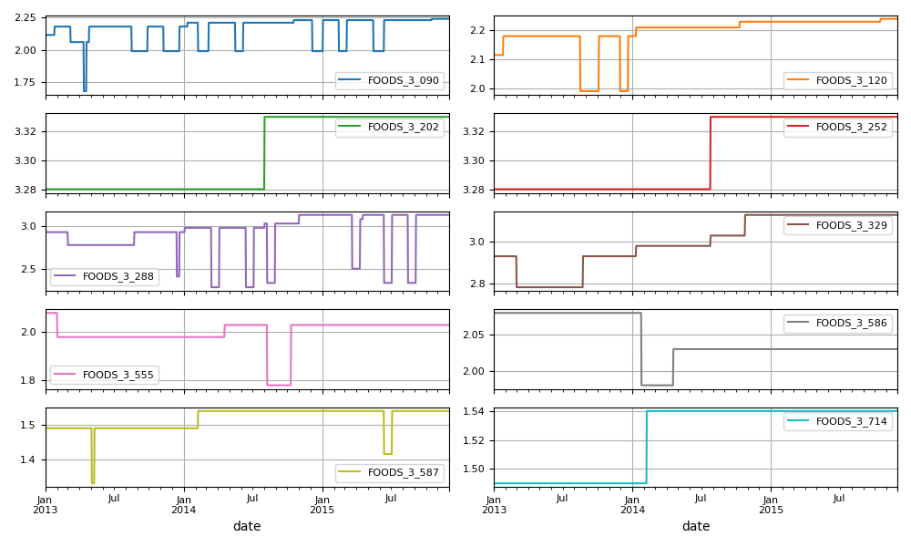
• Q6: How have the selling prices for each product changed over time?
• Q7: Are the selling prices fixed, or are they adjusted based on seasonality?
• Q8: How is the selling price impacted by seasonality?

Regarding events:

• Q9: How do major events throughout the year affect sales? Which holidays or festivities have the most significant impact?
• Q10: How does each event category influence sales?
• Q11: Which products are particularly affected by these special occasions?

6.2 Some results obtained through the EDA

These are some of the results that we have obtained by performing the exploratory Data Analysis (EDA) for both categorical and numerical variables that are present in the dataset.

A more detailed analysis of this stage can be found here.

6.3 Insights obtained through the EDA

Once the exploratory data analysis has been conducted, the following insights have been obtained:

Sales:

• Insight 1: New products were added after a few months, initially launched in just one store.
• Insight 2: One store is more significant, often used to test new products before they are introduced in the second store.
• Insight 3: There are periods when certain products experience zero demand. It is unclear whether this is due to stock-outs or simply a lack of sales during those times.
• Insight 4: Product performance is influenced by seasonality. Some products perform better in summer, while others do better in winter.
• Insight 5: Saturdays and Sundays consistently show the highest sales across all products.

Sell price:

• Insight 6: Selling prices show high variability, especially for certain products.
• Insight 7: Discounts are relatively common for some products.
• Insight 8: While some products have seen consistent price increases, others have experienced permanent price reductions. However, the majority of products maintain relatively stable prices.

Events:

• Insight 9: Sales per product tend to increase during special events, with Thanksgiving, Labor Day, and Easter performing particularly well.
• Insight 10: All event categories show similar performance, though sporting and cultural events generate slightly higher sales on average.

6.4 Recommended actions

Some of the actionable initiatives that the company can implement are the following:

1. With the current information, it is challenging to determine whether intermittent demand is due to stock-outs or simply zero demand for the product. Therefore, it is highly recommended to track warehouse data closely.

2. To optimize sales and reduce warehouse costs, implementing a forecasting model based on machine learning algorithms can be highly effective. A bottom-up approach, starting at the product level, is particularly recommended in this context.

3. Discounts have proven to be quite successful, especially for product 090, which is the top seller. It may be worthwhile to apply this strategy to other products and evaluate the overall impact.

4. Saturdays and Sundays show the highest sales volumes, presenting an opportunity to develop targeted strategies and campaigns.

5. Special days like Thanksgiving, Labor Day, and Easter generate significant sales. These occasions should be thoroughly analyzed, and marketing strategies should be developed to enhance the company’s profitability.

7. Variable creation and transformation

At this stage of the project, various variable transformation techniques are applied to ensure they meet the requirements of the algorithms used in the modeling phase.

First, to enhance the model’s predictive capacity, new variables are introduced, including:

• Intermittent demand variables: These variables estimate stock-outs using a rolling feature. It assumes that after a certain number of days with zero sales, a stock-out has occurred. Variables are created to account for fixed stock-outs over 3, 7, and 15 days.

• Lag variables: Lag variables are generated for sales (over a range of up to 15 days), selling price (over a range of up to 7 days), and stock-outs (over a range of up to 1 day). The one-day lag for stock-outs is chosen due to the nature of the variable. Since predicting exact zero demand is challenging for the model, using longer lags would be less effective, making a 1-day lag sufficient for this approach. These lag variables are particullarly useful in forecasting predictive models.

• Rolling windows variables: Rolling window variables for the minimum, average, and maximum values are created over a range of up to 15 days. These rolling variables have demonstrated strong predictive power in forecasting projects.

Note that all of these defined variables need to be shifted by one day in the functions, as the model cannot access information for the day it is predicting.

On the other hand, one-hot encoding and target encoding techniques are used to transform categorical variables into numerical ones. Both methods are applied at this stage: one-hot encoding serves as the basic transformation, while target encoding incorporates sales information before the transformation. We will experiment with both and select the most predictive approach during model analysis.

Regarding the numerical variables, no transformations are necessary since we are using LightGBM, a tree-based algorithm known for its effectiveness in forecasting projects with large datasets. As such, normalization and rescaling are not required for this project. Similarly, discretization or binarization of variables is not useful for this project, as our primary focus is on the model’s forecasting accuracy rather than interpretability. Class balancing is also not applicable in this context.

More details can be found here.

8. Forecasting model

At this stage, after completing data quality checks, exploratory data analysis, and variable transformation, we are ready to develop the forecasting model. As mentioned earlier, a supervised machine learning model will be used for this purpose, specifically the LightGBM algorithm, which has demonstrated strong performance in forecasting projects.

To develop the final forecasting model, we need to create a specific model for each product sold in each store. This requires building 20 independent models and reconciling the information using the bottom-up strategy mentioned earlier. The approach involves first testing a particular case to determine the optimal specifications. Then, in the final code, a loop will be implemented to apply the best parameters obtained for that specific product-store combination.

More details about this process can be found here.

8.1 General variable selection

A general variable selection process, considering all products in the dataset, is conducted at this stage of the project. The most predictive features are identified by comparing the results of three different selection methods: Recursive Feature Elimination, Mutual Information, and Permutation Importance. Among these, the Mutual Information method has demonstrated the best performance, offering a smooth transition between variables. This is crucial because we do not want to eliminate too many variables, as this selection analysis will need to be performed for each specific product-store combination.

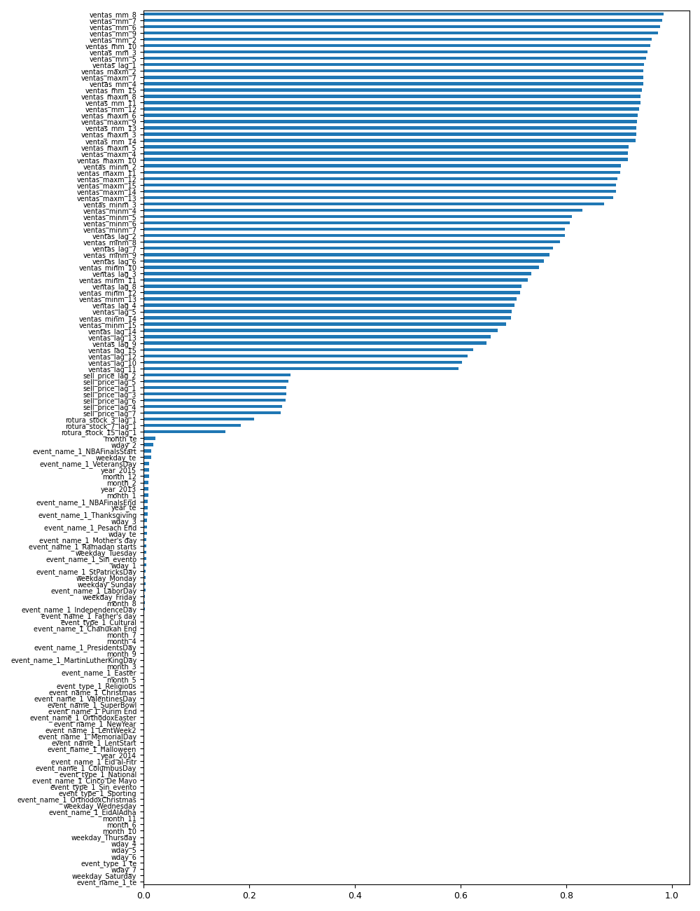
As a result of this analysis, a number of 73 variables have been selected. This number of variables will be used when applying the Mutual Information method to each product-store combination.

More information is provided here.

8.2 Developing a one-step forecasting model for a specific product-store combination

The objective at this stage of the project is not to produce the final models, but to design the modeling process—covering algorithm selection, hyperparameter optimization, and model evaluation—at the minimum analysis unit (product-store). This is done to ensure the process functions correctly and to identify and eliminate potential error sources before scaling the one-step forecasting process to all product-store combinations.

For this case, the product with code 586 sold in the store CA_3 is selected for this specific analysis.

Cross-validation strategy:

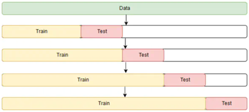
To prevent overfitting and evaluate model performance more robustly than with a simple train-test split, a cross-validation strategy has been implemented. However, cross-validation for time series data is not straightforward. Randomly assigning samples to the test or train sets is not feasible due to the temporal dependency between observations. The time sequence must be preserved.

The appropriate method for cross-validating time series models is rolling cross-validation. This approach starts with a small subset of data for training, forecasts subsequent data points, and then assesses the accuracy of these forecasts. The forecasted data points are incorporated into the next training set, and the process continues with forecasting subsequent data points.

In the present project the cross-validation process has been implemented using sklearn.model_selection.TimeSeriesSplit class of scikit-learn package with 3 splits and 8 days as maximum training size.

Selecting algorithm and hyperparameters:

As outlined in the general design phase of the project, the LightGBM algorithm is chosen for implementing the various models due to its strong balance between predictive accuracy and computational efficiency.

Different combinations of hyperparameters have been tested to find those with the best performance. Evaluation scores obtained in the tested parametrizations remains stable during the cross-validation process, which is a good indicator of the stability of the model predictions.

In the particular case of product 586 sold in store CA_3, the best parametrization obtained for the LightGBM algorithm is:

• learning_rate = 0.1
• max_iter = 100
• max_leaf_nodes = 31
• max_depth = None
• min_samples_leaf = 20
• l2_regularization = 0
• max_bins = 255
• scoring = ’loss'

Checking:

The objective here is not to evaluate the model’s quality, as the predictions were made using the training data, but rather to ensure that the process functions correctly. We aim to confirm that the predictions are within the correct order of magnitude and that no other anomalies are detected before moving forward with the project.

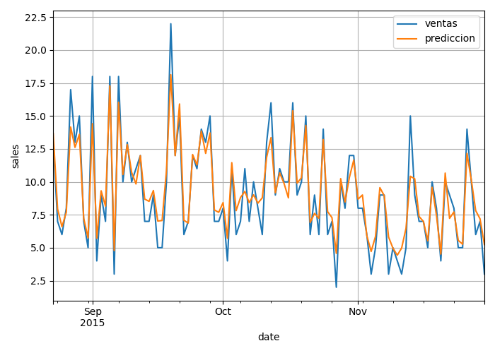
No issues have been identified, so the project will proceed as planned.

8.3 Generalizing the one-step forecasting model creation process

Once the forecasting model has been created and tested for an individual product-store combination, we can develop the necessary code to scale this process across all product-store combinations (massive forecasting evaluation). At this stage, the same 73 variables selected for product 586 are still being used. These variables will be updated to the specific ones for each combination in the final production code. The model algorithms, however, are now tailored to each specific combination.

Checking:

Again, it is important to note that the results obtained here are solely for verifying that the process functions correctly, not for evaluating the quality of the models, as predictions are made using the training data rather than the validation dataset.

No issues have been identified and the project can continue.

8.4 Multi-Step Forecasting

Once the general code for production is developed, it is essential to decide on the type of multi-step forecasting to implement. There are two main approaches to this: a direct forecasting and a recursive forecasting.

Direct Multi-step Forecasting:

In direct forecasting, separate models are trained for each future time step. For example, to predict the next 3 days, you would need to train three distinct models: one for t+1, another for t+2, and a third for t+3.

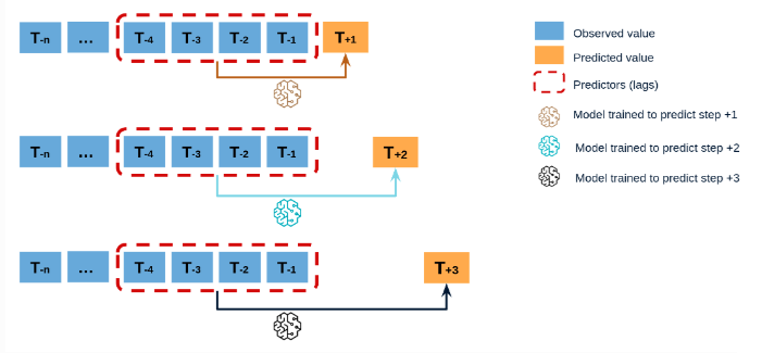
This approach allows each model to be tailored to the specific characteristics of the prediction horizon, often resulting in more accurate predictions for the individual time steps since each model is directly optimized for that step using only real data. However, this method requires more computational resources because multiple models need to be trained, and there is no shared information across different days, which can be a disadvantage if the time steps are strongly correlated.

Recursive Multi-step Forecasting:

In recursive forecasting (also known as iterative forecasting), a single model is used to predict one time step ahead, and this prediction is then fed back into the model to predict the next time step, and so on. For example, to predict t+1, t+2, and t+3, the model first predicts t+1, then uses the predicted t+1 to predict t+2, and uses t+2 to predict t+3.

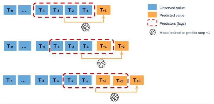
This approach is simpler as it requires only one model, reducing both training time and computational resources. It can also be more stable in some cases by leveraging the sequential nature of time series data. However, errors tend to propagate, leading to decreased accuracy for predictions further into the future. Additionally, the model is not specifically optimized for each time step beyond the first one.

For this project, a recursive multi-step forecasting approach has been implemented to minimize development and maintenance costs for the models."

9. Evaluation of the forecasting model

Once the general production code is developed, the forecasting model’s performance can be evaluated. To do this, we first need to prepare the data for the model. In real-life operation, the model requires only the last 15 days of data to function, as determined by the lag variables defined earlier in the modeling process. To facilitate this, we have prepared a file called ‘DatosParaProduccion.csv,’ which is part of the validation data (December 2015) reserved at the beginning of this project specifically for the evaluation of the final forecasting model.

In a real-life scenario, data will typically be sourced from a SQL database. The process should follow these steps:

• A SQL script should be prepared to extract the company’s last 15 days of data, with additional commands to structure the resulting CSV file. The output file must match the structure of ‘DatosParaProduccion.csv’ to ensure the forecasting model operates correctly.

• The CSV file is then generated and passed to the model to obtain predictions for the next 8 days.

• This process is repeated automatically each day to provide new predictive data, enabling informed business decisions that enhance the company’s profitability.

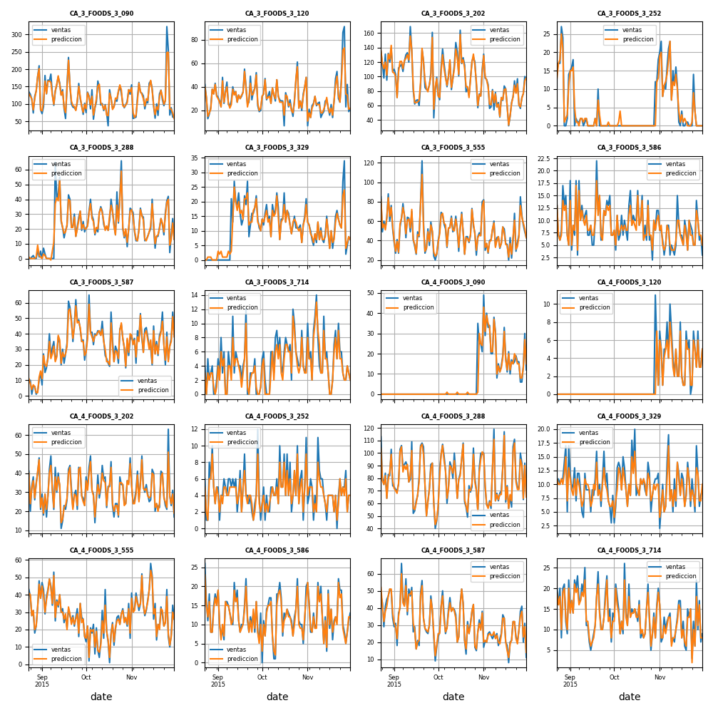
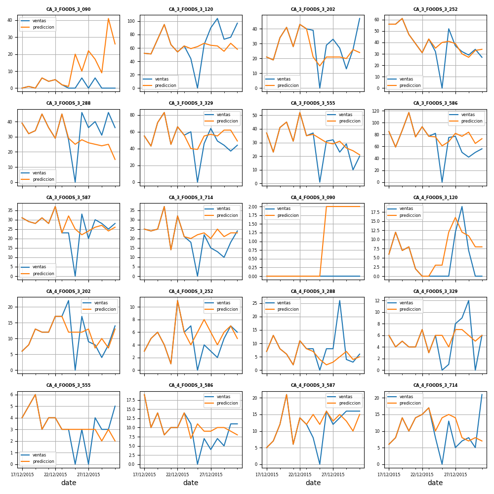
Therefore, the model has been evaluated using the prepared data in ‘DatosParaProduccion.csv,’ and the predictions for each product-store combination are shown in the figure below. While some models perform better than others, the overall performance of the recursive forecasting approach is satisfactory. The final mean absolute error, calculated by comparing actual and predicted sales across all product-store combinations, is approximately 4.73.

The evaluation results can be found here.

10. Retraining and Production scripts

After successfully developing, training, and evaluating the forecasting model, the final stage of the project involves organizing and optimizing the entire process. This is accomplished by compiling all necessary processes, functions, and code into two streamlined Python scripts:

• Retraining Script: This script is designed to automatically retrain all developed models with new data as needed, ensuring that the models remain accurate and up-to-date.

• Production Script: This script executes all models and generates the desired results, ensuring a smooth transition from development to production.