Risk Scoring for a Neobank Company

Note: Documentation available on the GitHub Repository is currently in Spanish. It will be soon updated to English.
Table of Contents
1. Introduction
The client for this project is a neobank specializing in offering competitively priced loans. However, the company is concerned about the quality of borrowers accessing their products. They require a robust system to assist in making informed loan approval decisions based on applicants’ profiles.
The goal is to implement a risk-scoring model using artificial intelligence algorithms to identify ‘risky’ applicants and estimate their associated expected losses. This information will be used to manage the bank’s economic capital, portfolio, and risk assessment effectively.
Notes:
- This article presents a technical explanation of the development process followed in the project.
- Source code can be found here.
- You can also test the Risk Scoring Analyzer web application.
2. Objectives
The main objective is to develop a risk-scoring model using machine learning algorithms to predict potentially risky borrowers. This model will estimate the expected financial loss for each new customer-loan pairing, based on the company’s historical data. By leveraging this advanced analytical tool, the company’s performance will be significantly enhanced.
3. Understanding the problem
Credit risk is associated with the possibility that a borrower will fail to meet their obligations according to the agreed terms, such as repaying a loan. This risk is a critical concern for banks because it can lead to financial losses if borrowers default on their loans. Banks manage credit risk through various means, including:
Credit Assessment: Evaluating the borrower’s creditworthiness before approving a loan.Diversification: Spreading out lending across different sectors and borrowers to reduce the impact of any single default.Collateral: Requiring assets to secure loans, which can be seized if the borrower defaults.Monitoring: Continuously assessing borrowers’ financial health and adjusting terms as needed.
Effective credit risk management is crucial for banks to maintain financial stability and absorb potential losses without compromising their overall health. In this regard, machine learning algorithms have proven particularly valuable. They can be employed to develop sophisticated models that predict financial loss per borrower using data science techniques and historical company data. These advanced models enhance the accuracy of risk assessments and support better decision-making in credit management.
4. Project Design
4.1 Methodology
The project has been designed with a multi-step methodology, which is summarized in the figure bellow.
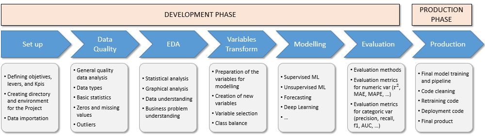
The process for this project consists of two main stages: the development phase and the production phase.
The development phase begins with the set up and data importation, followed by a thorough data quality review. Next, an exploratory data analysis is conducted to uncover key insights. The variable transformation step involves selecting the most relevant variables that impact the problem and applying the necessary transformations. Following this, the risk-scoring model is implemented based on machine learning algorithms. During the evaluation process, all metrics are thoroughly tested.
In the production phase, the model is prepared for deployment, ensuring that the code is optimized for production. Additionally, a retraining script is created during this stage to facilitate future updates.
4.2 Project scope
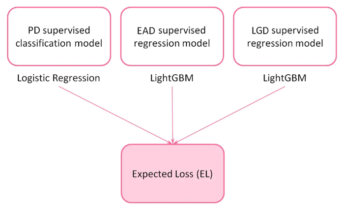
To estimate the Expected Loss (EL) associated with a loan application, three key risk parameters are considered:
Probability of Default (PD): This measures the likelihood that a borrower will default, based on an internally assigned credit rating.Exposure at Default (EAD): This indicates the amount of outstanding debt at the time of default.Loss Given Default (LGD): This metric represents the percentage of the loan exposure that is not expected to be recovered if a default occurs.
To estimate these risk parameters, three predictive machine learning models will be developed. The predictions from these models will then be combined to calculate the expected loss for each loan transaction. To calculate this value, the following formula is applied:
$$ \textup{EL}[$] = \textup{PD} \cdot \textup{P}[$] \cdot \textup{EAD} \cdot \textup{LDG}, $$where P is the loan principal, i.e., the amount of money the borrower whises to apply for.
4.3 Entities and data
The data under analysis includes information collected by the company about two primary entities:
Borrowers: This dataset features details on the applicant’s profile, such as employment history, the number of mortgages and credit lines, annual income, and other personal information.Loans: The remaining features provide information about the loans themselves, including the loan amount, interest rate, status (i.e., whether the loan is current or in default), tenor (either 36 or 60 months), among other details.
On the other hand, before conducting any analysis or data transformation, it is crucial to set aside a randomly selected portion of the dataset for validation purposes. This reserved data will be used to validate the models after they have been trained and tested on the remaining data.
5. Data Quality
In this stage of the project, general data quality correction processes have been applied, such as:
- Data renaming.
- Type correction.
- Proper selection of the most relevant data for the project.
- Analysis of nulls and duplicated registers.
- Analysis of numerical and categorical variables.
- Discretization of variables.
- Creation of new variables.
The entire process can be consulted in detail here.
6. Exploratory Data Analysis
The aim of this phase of the project is to identify trends and patterns that can be transformed into insights, providing valuable information for our project. To achieve this, we perform various statistical evaluations and create graphical representations.
In order to guide this process, a series of seed questions are proposed to serve as a basis for the analysis.
6.1 Seed questions
Regarding borrowers:
Q1: What are the most common professions among clients applying for loans?Q2: How effective is the score feature assigned by the company in evaluating each applicant?Q3: Can different customer behavior profiles be identified based on how they use their credit cards?Q4: How do factors like income and debt-to-income ratio impact the borrower’s profile?
Regarding loans:
Q5: Are there differences in the percentage of late payments and charge-offs between 36-month and 60-month loans?Q6: Are certain loan purposes more likely to default than others?Q7: What type of interest is applied to the loans? how is it related to the borrower’s profile?
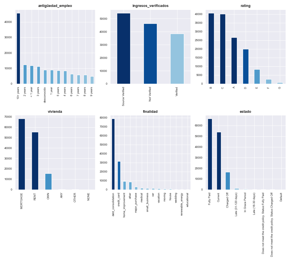
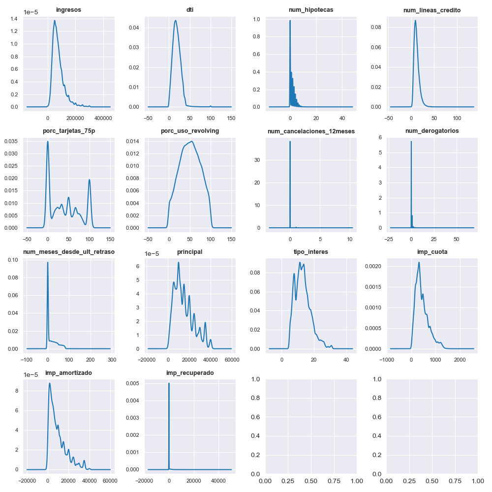
6.2 Some results obtained through the EDA
These are some of the results that we have obtained by performing the exploratory Data Analysis (EDA) for both categorical and numerical variables that are present in the dataset.
A more detailed analysis of this stage can be found here.
6.3 Insights obtained through the EDA
Once the exploratory data analysis has been conducted, the following insights have been obtained:
Borrowers:
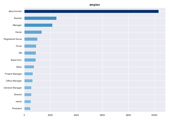
Insight 1: Borrowers with poorer credit scores tend to borrow larger amounts and have lower annual incomes compared to those with higher credit scores. As a result, they face higher monthly installments and interest rates.Insight 2: One-third of all customers have been employed for more than 10 years, though the job titles of many clients remain unknown. Among those who do provide this information, the top three most common occupations are ‘Teacher,’ ‘Manager,’ and ‘Owner.’Insight 3: The credit score feature is predictive of loan outcomes: the percentage of loans charged off increases as borrowers’ credit scores decrease, while the percentage of fully paid loans rises with higher credit scores.Insight 4: Three main groups of borrowers can be clearly distinguished based on their credit card usage: those who use less than 20% of their available credit, those who use between 20% and 80%, and those who use more than 80% of their available credit.
Loans:
Insight 5: In general, 60-month loans tend to have a higher percentage of late payments and charge-offs.Insight 6: Loans for ‘moving’ and ‘small business’ purposes have a slightly higher charge-off rate (16%-17%) compared to the average for other loan purposes, which is around 11%.Insight 7: The types of interest range from 5 to 31%, with the mayority of them falling below 16%.
6.4 Recommended actions
Some of the actionable initiatives that the company can implement are the following:
Credit scores appear to be effective in identifying high-quality borrowers. These profiles should be targeted for promotion, and a broader range of products, such as investment opportunities, stocks, and index funds, could be offered to them.
The job title category needs improvement to provide more accurate information, which will be beneficial for the development of the machine learning algorithms.
Since three main borrower profiles have been identified based on credit card usage, targeted campaigns can be developed for each group. Customized products or loans tailored to their specific needs could be offered to them.
According to the company’s historical data, 30-month loans are performing better. These should be promoted, and additional products in this category could be considered.
7. Variable creation and transformation
At this stage of the project, various variable transformation techniques are applied to ensure they meet the requirements of the algorithms used in the modeling phase.
It is important to note that creating the risk-scoring model, which predicts the Expected Loss associated with each loan application, requires developing three separate models: one for the Probability of Default (PD), another for the Exposure at Default (EAD), and a third for the Loss Given Default (LGD). To achieve this, we need to create distinct target variables for each model:
Target for PD model: This target is created by analyzing the ’estado’ category. Records with values such as ‘Charged Off’, ‘Does not meet the credit policy. Status: Charged Off’, and ‘Default’ are considered defaults and are marked with a ’target_pd’ of 1. The rest of records are marked with 0. In addition, this target is categorical so a supervised classifier machine learning model will be used.Target for EAD model: This target is determined by calculating the ratio between the outstanding amount and the original loan amount, as defined by the following formula:
Target for LGD model: This target represents the amount that is not recovered in the event of a default, as defined by the following formula:
On the other hand, one-hot encoding and ordinal encoding techniques are used to transform categorical variables into numerical ones. At this stage, both methods are applied: one-hot encoding is used for basic transformations, while ordinal encoding is applied to variables with a hierarchical structure, such as profile ratings and length of employment.
Additionally, the text data in the ‘descripcion’ variable is analyzed using the TfidfVectorizer technique. This method converts a collection of text documents into a matrix of TF-IDF (Term Frequency-Inverse Document Frequency) features. TF-IDF reflects the importance of a word within a document relative to the entire dataset, reducing the weight of commonly used words. This approach is commonly used in text classification and clustering to capture the relevance of terms. However, no relevant terms were identified using this method, so it was ultimately not adopted in this project.
Regarding the numerical variables, binarization is applied to the ’num_derogatorios’ variable, and rescaling is applied to the remaining ones. Specifically, the MinMaxScaling technique is used, as it rescales data within a 0 to 1 range, which is more precise for this particular project. Other techniques, such as discretization, normalization, or class balancing, are not applicable in this context.
More details can be found here.
8. Risk-scoring model
At this stage, after completing data quality checks, exploratory data analysis, and variable transformation, we are ready to develop the risk-scoring model. As mentioned earlier, this model is compound of three different and independent algorithms: a first one for the Probability of Default, a second one for the Exposure at Default, and a third one for the Loss Given Default.
It is important to note that the model for estimating the Probability of Default will utilize a logistic regression algorithm. ‘Black box algorithms’ are often unsuitable for regulated financial services due to their lack of interpretability and auditability, which can pose macro-level risks and, in some cases, conflict with legal requirements for explainability. To address this, a highly explainable AI model like logistic regression will be used, as it provides clear and understandable insights into its decision-making process.
For estimating Exposure at Default and Loss Given Default, various algorithms and hyperparameter combinations were evaluated, including Ridge, Lasso, and LightGBM. Ultimately, the LightGBM algorithm was selected for both cases due to its superior performance.
On the other hand, it is important to highlight two main types of scoring analysis:
Acquisition: Acquisition models, like the one used in this case, are designed to analyze new clients. As a result, the pool of variables available is much more limited, leading to generally lower performance and less favorable validation metrics.Behavioral: Behavioral models are used to track and analyze how a client’s profile evolves over time. These models leverage a much larger pool of variables, resulting in superior overall performance.
Since we are working within an acquisition context, the expected validation metrics are not as high as those in behavior models. For example, an AUC around 0.7 is considered decent in this type of analysis. Additionally, no general variable selection is applied here because the already limited pool of variables would be further reduced, which would not benefit the model’s development.
8.1 Probability of Default (PD) model
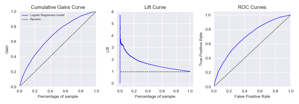
As previously mentioned, a supervised classifier machine learning algorithm is used for the PD model. Particularly, a logistic regression is selected due to its high interpretability. Additionally, appropriate regularization is included in the hyperparameterization to help select the most relevant variables, as no general variable selection was applied in the previous step. All combinations are alse tested using the cross-validation method to ensure the model’s stability. The model’s performance is evaluated using three methods: the cumulative gains curve, the lift curve, and the ROC curve.
In simple terms, the cumulative gains curve measures the effectiveness of a classification model by showing the proportion of true positives identified, while the lift curve indicates how much better the model performs compared to random guessing, illustrating the model’s added value. The ROC curve evaluates the trade-off between the true positive rate (sensitivity) and the false positive rate across various threshold settings.
The cumulative gains and lift curves focus on the model’s ability to identify positives within a ranked population, while the ROC curve assesses the model’s overall discriminatory power across all thresholds. The results are shown in the figure below.
The best hyperparametrization found for the logistic regression algorithm is the following:
- C = 1
- n_jobs = -1
- penalty = ’l1’
- solver = ‘saga’
The model achieved a final AUC of 0.699 after being trained and validated against the test dataset.
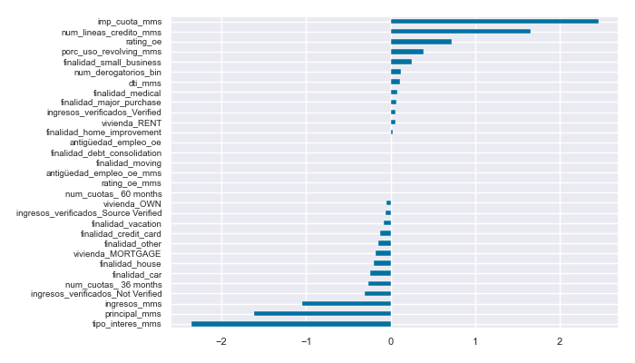
Additionally, an analysis of the coefficients from the trained logistic regression model reveals that the factors most strongly influencing the customer’s probability of default are the type of loan interest, loan amount, annual income, number of credit lines, and the monthly payment amount.
More information is provided here.
8.2 Exposure at Default (EAD) model
For the EAD model, supervised regressors machine learning algorithms are required. In this case, different combinations of linear regression algorithms (Ridge, Lasso) are tested against the tree-based LightGBM algorithm, each with various hyperparameter settings. It is found that the LightGBM architecture performs the best. Since interpretability is less critical for the EAD model and due to the significant performance difference between these algorithms in this case, LightGBM is ultimately adopted, as mentioned in previous steps. The final adopted hyperparametrization for the LightGBM algorithm is the following:
- learning_rate = 0.1
- max_iter = 200
- max_depth = 20
- min_samples_leaf = 100
- scoring = ’neg_mean_absolute_percentage_error’
- l2_regularization = 1
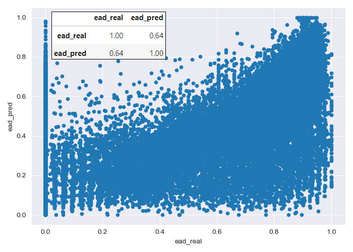
As it is shown in the figure above, the model’s error in predicting the level of unpaid loan balance at the time of default is relatively high. However, it is important to note that errors in risk acquisition models (like this one) are generally much higher than in behavioral models, marketing, or customer management models, as significantly less customer information is available.
Additionally, it is important to remember that the model is designed to predict outcomes for both defaulting and non-defaulting borrowers, as this information is not available for new customers. Consequently, the model often attempts to predict the exposure at default for borrowers who are unlikely to default, which also contributes to the higher error rates observed in the modeling process.
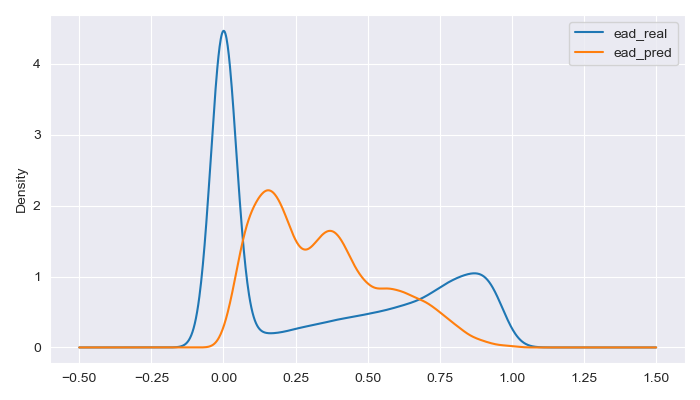
In the real data, it can be identified three distinct groups of borrowers: a majority group with zero exposure at default, a second group with intermediate exposures (0.25-0.75), and a final group consisting of borrowers with high exposure at default.
The model’s predictions tend to cluster around intermediate default exposures, leading to larger errors when predicting borrowers with very low or very high actual default exposures.
For customers who will have very limited exposure at default, the model predicts some degree of exposure, resulting in slightly higher fees or interest charges than they would otherwise be entitled to.
On the other hand, for customers with high actual default exposures, the model tends to predict lower exposure levels, leading to lower fees or interest being applied than would be appropriate.
However, from a business perspective, the model’s overall performance is quite acceptable. It balances the fees and interest not collected from borrowers who end up with high default exposures by applying additional charges to those customers who ultimately do not default, thereby covering the aggregate risk of the client portfolio.
More information is provided here.
8.3 Loss Given Default (LGD) model
For the LGD model, supervised regression machine learning algorithms are once again required. Similar to the EAD model, various combinations of linear regression algorithms (Ridge, Lasso) are compared against the tree-based LightGBM algorithm, each with different hyperparameter settings. The results are similar to those obtained for the EAD model, with the LightGBM algorithm demonstrating significantly better performance. As in the previous case, interpretability is less critical for the LGD model, and due to the substantial performance difference between these algorithms, LightGBM is ultimately adopted. The final hyperparameter configuration for the LightGBM algorithm is as follows:
- learning_rate = 0.1
- max_iter = 200
- max_depth = 20
- min_samples_leaf = 100
- scoring = ’neg_mean_absolute_percentage_error’
- l2_regularization = 0.25
The error for this model is slightly higher than that of the EAD model, which can be attributed to the same reasons previously discussed, with the added factor of greater polarization in the data.
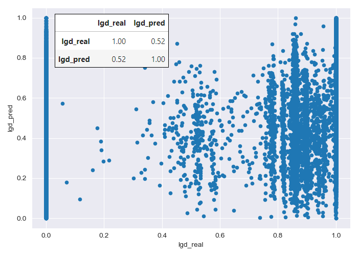
In the real data, two large groups can be distinguished:
A group of loans where no amount is recovered, either because the borrower has not defaulted or because the borrower has defaulted but the bank has been unable to recover any funds.
A second group of loans where the full amount has been recovered, either because the borrower has fully repaid the loan or because the bank was able to recover the full amount despite a default.
The model’s predictions tend to gravitate toward intermediate loss levels, resulting in larger errors when predicting loans that are either fully recovered or entirely lost.
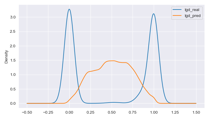
However, as discussed with the EAD model, the LGD model’s performance is still acceptable at an aggregate level from a business perspective. It compensates for the fully lost loans by predicting a loss level between 25% and 75% for most customers, including those who ultimately repay their loans in full, thus covering the overall risk of the client portfolio.
More information is provided here.
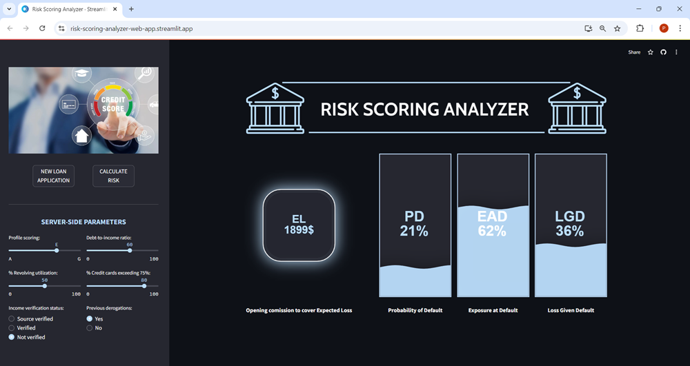
8.4 Final Expected Loss (EL) model
Once the PD, EAD, and LGD models have been developed, the Expected Loss (EL) for each new loan application is obtained by simply combining the predictions of these models and the principal amount of the loan as discussed in the project scope section.
$$ \textup{EL}[$] = \textup{PD} \cdot \textup{P}[$] \cdot \textup{EAD} \cdot \textup{LDG}. $$9. Evaluation of the risk-scoring model
Once the general production code is developed, the performance of the risk-scoring model can be evaluated. To do this, the model is tested on a batch of 60000 new loan applications that were never used before, corresponding to the validation dataset reserved at the beginning of the project. The results are displayed in the scatterplot above.
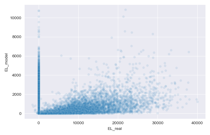
As shown in the figure, the results are not ideal. The EL model is struggling to accurately predict some non-defaulted borrowers, assigning them higher loss values than appropriate. Conversely, it also fails to predict certain real losses by assigning them very low values. This poor performance at both extremes is due to the nature of the data, with high polarization, particularly in the LGD model, being the primary cause of this issue.
However, the EL model remains useful for selecting and differentiating loan applications. The denser region of the chart, where more cases are concentrated (and where more applications are likely to fall), performs better, making the model valuable in practical scenarios.
By implementing this developed risk-scoring model, the neo bank will be able to make more informed decisions about loan applicants. This will enable the bank to more effectively manage its economic capital, client portfolio, and risk assessment processes, ultimately improving the company’s performance and increasing profitability.
The evaluation results can be found here.
10. Retraining and Production scripts
After successfully developing, training, and evaluating the forecasting model, the final stage of the project involves organizing and optimizing the entire process. This is accomplished by compiling all necessary processes, functions, and code into two streamlined Python scripts:
Retraining Script: This script is designed to automatically retrain all developed models with new data as needed, ensuring that the models remain accurate and up-to-date.Production Script: This script executes all models and generates the desired results, ensuring a smooth transition from development to production.
11. Model deployment. Web app creation
To maximize the value of the developed machine learning models, it is essential to seamlessly deploy them into production so that employees can start utilizing them to make informed, practical decisions.
To achieve this, a prototype web application has been designed. This web app gathers internal data from the company for each client, as well as information provided by the borrower through their loan application.
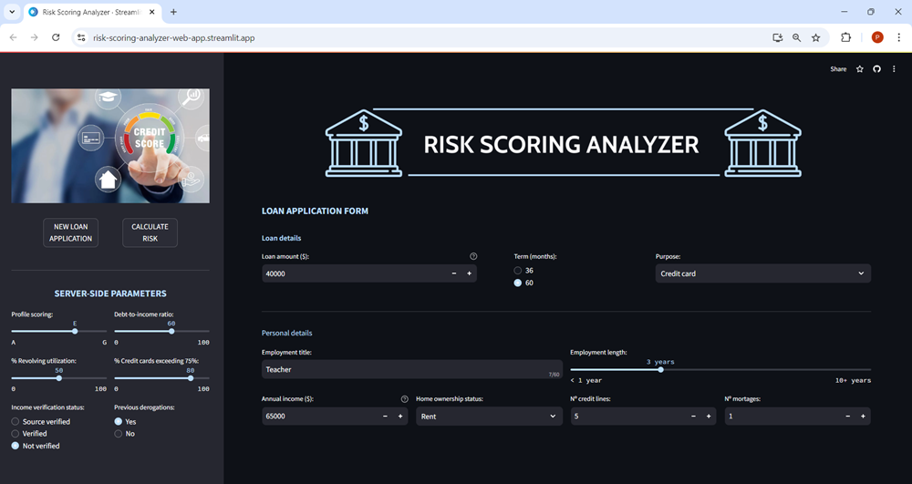
Once the data is entered, users can click the CALCULATE RISK button, which triggers the machine learning models to process the data. The application will then return the Expected Loss for the loan application, along with key performance indicators such as the Probability of Default, Exposure at Default, and Loss Given Default.
The necessary files for the creation of the web app can be found here.
Pablo Esteban
Data Scientist and PhD in Mechatronics. I’m passionate about solving problems and optimizing processes, especially those related to coding and business knowledge.